Large language models are increasingly being used as data analysts. Give an LLM a CSV and ask, “What is driving customer churn?” It will return a confident answer. 

But is it actually analyzing your data? Or is it replaying patterns from thousands of Kaggle notebooks and textbook datasets it encountered during training? 

SleuthBench (Statistical LLM Evaluation Using Tabular Hidden Signals) is our attempt to answer that question rigorously. It is a benchmark for evaluating how well LLMs analyze tabular data, built around one simple idea: plant the answer in the data first, then ask the question.

We find that even frontier models struggle in this setup. With access to the raw table and a Python sandbox, the six models in our evaluation answered only 65% of the benchmark questions correctly, and prompts that described a business concern without naming the statistical mechanism were harder still.

We conclude by evaluating Intelligible’s empirical layer, built from its core interpretability stack. Adding it raised aggregate accuracy from 65% to 75% in our experiments.

1. Why Existing Benchmarks Are Not Enough

There is no shortage of work on tables and LLMs. But most existing benchmarks fall into two groups, and neither fully answers the question we care about: can an LLM answer analytical questions about real, messy data by analyzing the data itself? 

The first group is question-driven reasoning over tables, including WikiTableQuestions, TabFact, and TableBench. These benchmarks range from compositional question answering (where a complex question is broken down into simpler sub-questions) to fact verification. These benchmarks ask models to perform a specified task over a table. They do not directly test whether an agent can decide what analysis to run and uncover a hidden statistical signal. 

The second group is much closer to our goal: data analysis and data science benchmarks for AI agents. Examples include InfiAgent-DABench, DSBench, DA-Code, QRData,  and DiscoveryBench. These include a variety of more challenging tasks, such as data analysis, data modeling, coding for data science, quantitative reasoning, and data-driven discovery. 

These benchmarks share a structural limitation: the data is public, while the ground truth must be curated manually. In practice, this creates three problems. 

1. Ground truth is scarce. Questions such as “Which feature is most important?” or “Is there an interaction effect between feature A and feature B?” often have no single objective answer in real data. Human-derived ground truth is expensive and debatable. Every DiscoveryBench task requires someone to reconstruct an analysis from a paper. QRData includes multiple-choice and numerical questions with unique ground-truth answers, but more open-ended analytical questions—with several defensible interpretations—are difficult to include.
2. Data contamination is common. Many widely used public datasets have been seen in model training corpora. Bordt et al. found evidence that GPT-3.5 and GPT-4 had memorized several classic tabular datasets, including California Housing, Titanic, and Adult, and performed better on datasets seen during training. A model may approach the correct answer through memorization or domain priors without truly analyzing the table in front of it.
3. Static benchmarks decay. Once a benchmark is published, it begins leaking into future training data. LiveBench and LiveCodeBench address this decay by continually replacing old questions with new ones. For data-analysis benchmarks, however, that approach is especially expensive: each new question requires a new round of ground-truth curation.

SleuthBench takes a different route. It injects statistical phenomena that occur in real data into ordinary datasets. The construction process automatically creates the ground truth, and the same procedure can be applied to new datasets to generate new questions without another round of manual labeling. 

2. The Core Idea: Inject a Phenomenon, Then Ask About It

SleuthBench reverses the usual benchmark-building workflow. Instead of searching an existing dataset for interesting questions, we start with a dataset and inject a known statistical phenomenon into it: an inverted-U relationship between a feature and the target, a missing-like category whose membership depends on the target, or a column that quietly identifies corrupted rows. 

These are not arbitrary synthetic puzzles. Although the injected phenomena are crafted manually, they target patterns analysts encounter in practice: nonlinear feature effects and pairwise interactions observed in real datasets, missingness and imputation artifacts documented in clinical data, and downstream data-quality failures reported by practitioners. 

The injection is a controlled edit. Because the procedure is known, we know which feature changed, where a peak lies, and how strong the effect is. 

That single operation addresses all three problems above.

1. Construction determines the ground truth. Ground-truth answers are computed deterministically from the known injection parameters and the resulting table. No manual labeling is required, and no LLM participates in answer generation.
2. Contamination is substantially reduced. The edited table did not exist before we generated it, so memorizing the base dataset is not enough to recover the answer. The model must genuinely inspect the data.
3. New benchmark cases can be generated at scale. Apply the same reusable injection procedure to another compatible dataset, or vary the seed or effect strength, and the pipeline produces a new dataset–question pair. Each case records its seed, so it can be reproduced exactly with the same code version and input dataset.

Injection Validation

To ensure that an injected dataset actually contains the intended pattern, every generated case passes through a validation stage. Analytical checks verify that the planted phenomenon meets predefined detectability criteria and rule out competing patterns. Cases that fail validation are excluded before any evaluated model sees them. 

After validation, the ground truth is computed deterministically from the known injection parameters and the edited table. Depending on the phenomenon, those parameters identify the changed feature, the peak location, the corrupted rows, or another relevant effect.

Question Coverage

The question pool contains 18 different injections across four categories.

• Feature importance: Recover the correct feature-importance ranking or identify a feature that is pure noise with respect to the target.
• Shape functions: Find a feature with an inverted-U relationship with the target and locate its peak, identify the feature with the strongest non-monotone or V-shaped relationship, or find where the target changes abruptly or levels off.
• Interaction detection: Find the dominant feature interaction and determine its direction, or identify a pair that exhibits positive synergy or a reversal. For example, a promotional offer and free shipping might each lift sales on their own while combining them suppresses sales.
• Data quality: Find a column that identifies corrupted rows, detect anomalous records, recognize when the sample size is insufficient to determine that two groups are statistically distinct, find a category label that semantically encodes missingness, or detect a missingness pattern that is target-dependent.

We inject these phenomena into real datasets, so the resulting tables look just like data an analyst might encounter. 

Phrasing as an independent axis of difficulty

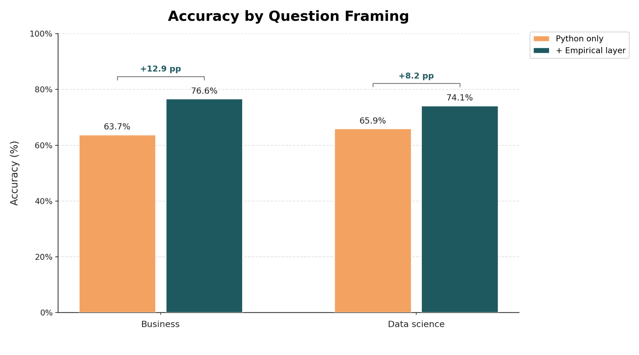
Each injection also defines two phrasings of the same question: a data-science version and a business version.  These phrasings represent two kinds of users. A data scientist who knows the mechanism to search for might ask, “Are any values in feature A imputed?” A business user might describe the same concern without naming the mechanism: “Is there any unusual pattern in feature A?” The injected dataset and ground-truth answer remain the same; only the framing changes. 

3. Giving the LLM an Empirical Layer

The key experimental variable in SleuthBench is which tools the model receives. 

In the baseline condition, the model gets a Python sandbox. It can load the CSV, explore the data with Python, and fit whatever models it wants. This is the “LLM as a junior data scientist” setup. 

The enhanced condition adds an empirical layer built from Intelligible’s core interpretability stack. For every injected dataset, we precompute the same suite of task-agnostic components.

• Explainable Boosting Machine (EBM) outputs, including feature-importance scores, feature-effect curves, and pairwise interaction surfaces.
• Per-column statistics and distribution profiles.
• Pairwise correlation and association measures.
• Missing-value and conditional-missingness patterns.
• Univariate and multivariate outlier reports.
• Feature descriptions, contexts, and encoding metadata.
• Dataset-level statistics and computation metadata.

With only the raw table and Python, the model must rediscover this structure through open-ended exploration. In practice, models often try a handful of analyses, settle on a plausible story, and stop.

The empirical components are generated uniformly for every dataset without consulting the benchmark question, the injection parameters, or the answer key. They make exploration more systematic and narrow the hypothesis space while leaving the model to select and interpret the relevant evidence.

4. Results: How Much Is the Empirical Layer Worth?

Evaluation Setup

The main goal of the evaluation is to measure how much access to Intelligible’s empirical layer improves an LLM’s ability to analyze data. To make this comparison fair, the model can write and run Python code in a separate sandbox in both conditions; the only difference is whether it also has access to the empirical layer.

Because LLMs are used for data analysis across many kinds of problems and by users with different levels of technical expertise, we evaluate performance along four dimensions.

• Statistical phenomena. The benchmark covers a range of patterns analysts encounter in real data, including feature importance, nonlinear effects, interactions, and data-quality issues.
• Data domains. The benchmark uses six real-world datasets spanning three different domains: manufacturing, transportation, and real estate. 
• Prompting styles. Each task is asked in both data-science language and business-oriented language, reflecting differences in the technical jargon that users may use when asking an LLM to analyze data.
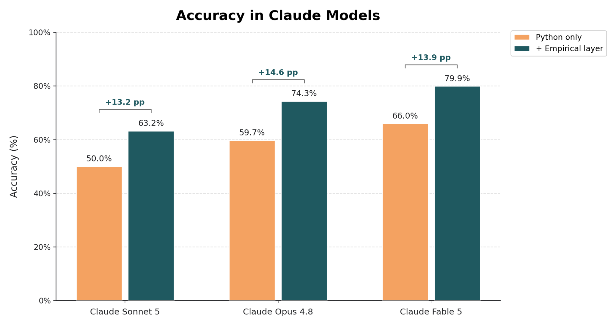
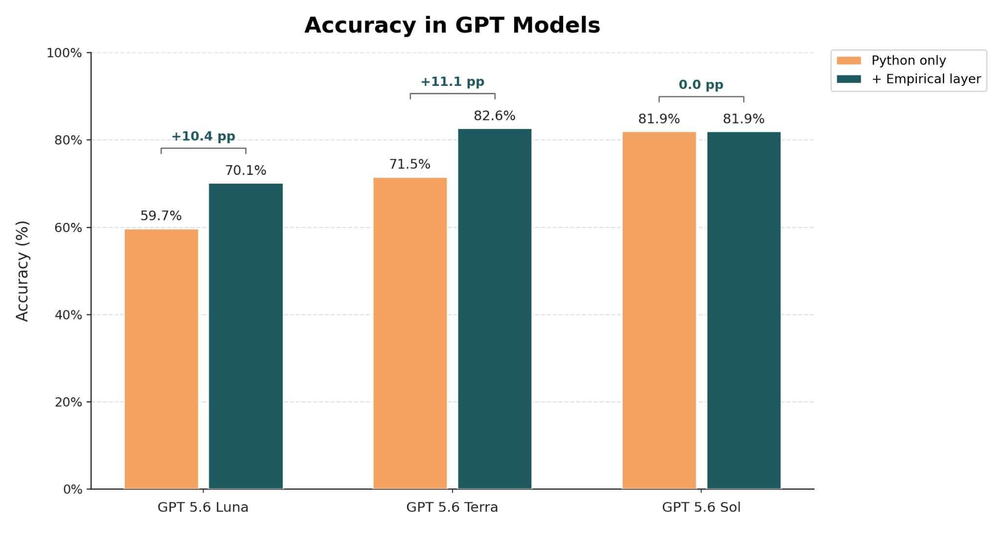
• Models. We evaluate six models, three Claude variants (Sonnet 5, Opus 4.8, and Fable 5) and three GPT-5.6 variants (Luna, Terra, and Sol).

Across these settings, we compare performance with Python alone against Python plus the empirical layer.

Overall Results

Across the benchmark, models answered 65% of questions correctly with Python alone. Adding the empirical layer increased accuracy to 75%.

The improvement is not limited to a single model or type of question. As we break down below, the empirical layer improves performance for nearly all models and the effect is especially pronounced when users describe a problem without naming the statistical mechanism they are looking for.

Results across models

The empirical layer helps almost every model we tested. Five of the six models improve by more than 10 percentage points, with the largest gain coming from Claude Opus 4.8. GPT-5.6 Sol is the odd one out: its overall score stays flat. But that aggregate result hides two opposing effects: Sol gets better on data-science questions and worse on business-style questions. And it does so by the same amount! In other words, the empirical layer still changes Sol’s behavior; the gains just cancel out in the aggregate.

Results across prompting styles

The same analytical problem can be phrased very differently depending on who is asking. A data-science prompt often names the statistical mechanism directly. A business-style prompt may describe the concern more broadly. In our benchmark, these paired questions use the same data and have the same correct answer; only the wording changes. 

The empirical layer improves performance regardless of prompting style, but its effect is much larger for business-style questions. When a prompt uses precise technical language, the model already has a strong clue about what analysis to run. Broader questions are harder: the model must first do some real sleuthing before figuring out what it should be looking for.

This is where the empirical layer helps most. Its structured view of the data makes relevant patterns easier to discover, even when the user cannot name the statistical mechanism in advance.

Case Study: How the Empirical Layers Guides the LLM to the Right Answer 

Aggregate results can hide a subtler failure mode: a model may perform substantial analysis and produce a statistically defensible answer, but it may do so while using a definition of the statistical phenomenon of interest that is at odds with the definition used by the benchmark. We now discuss a specific example to see how this may arise.

Original dataset.

The original dataset records traffic volume against a variety of features such as weather and seasonality. For this case study, we restrict our attention to a sample of 1,000 rows. Four of its columns are of interest:

• temp, the temperature,
• month, the month of the observation,
• weather_description, a categorical column with 28 weather categories (such as “light rain”, “Sky is Clear”, or “thunderstorm”), and
• traffic_volume, which is considered as the target., 

Injection Procedure 

The injection planted an interaction between month and temp such that two things occur: when either of these features is large, but not the other, then the traffic volume is high; and when both features are large, then the traffic volume is lower. This is a surprising interaction that often occurs in real datasets: two features are beneficial in isolation but detrimental when combined.

Question 

“Which two columns look fairly ordinary when considered separately but reveal the strongest unusual pattern in traffic_volume when looked at together? Return the two column names as: column_a, column_b. “

As described above, the expected answer is “month, temp”.

The two reasoning trajectories

In this case study we consider how GPT-5.6 Luna reasoned through this question, either using only Python or using both Python and the empirical layer.

Trajectory with Python only

GPT-5.6 Luna explored the data through several different interaction proxies and it ultimately selected weather_description and month. 

This is because the model used uncorrected empirical mutual information as its definition of interaction. Viewed through that lens, the model’s erroneous answer is defensible: weather_description has 28 categories and month has 12, yielding as many as 336 joint cells for only 1,000 observations. Uncorrected empirical mutual information tends to favor high-cardinality combinations and can interpret sparse, locally extreme cells as strong interactions, which is exactly what happened here.

Trajectory with the Empirical Layer

With the empirical layer, the same model first inspected the schema and general metadata. It then retrieved target associations and compared six EBM interaction graphs. Among these candidates, the EBM interaction term between temp and month was the strongest interaction, and it is this pair that the model answered with. 

Comparing the two reasoning trajectories

Beyond accuracy, the empirical layer displays other benefits in this case. When using the empirical layer, the model used half as many input tokens and responded six times faster! Moreover, the reasoning trace of the model using the empirical layer is much easier to audit: without the empirical layer, the model performs a long sequence of exploratory tool calls running Python code, frequently changing how it defines an interaction; with the empirical layer, the model’s reasoning is anchored by a trusted piece of the empirical layer (in this case: EBM graphs).

The empirical layer did more than improve the final answer. It imposed a consistent, model-based definition of interaction and exposed comparable evidence for a bounded set of named pairs. By contrast, the Python-only trajectory moved among several plausible but non-equivalent ways of measuring interaction without committing to a single criterion for the final ranking. In future iterations of SleuthBench we will examine whether an empirical layer can improve not only accuracy, but also consistency across prompt phrasings and repeated runs.