What Really Drives Home Prices in King County

Blog

Joel Webb

August 24, 2026

What Really Drives Home Prices in King County

How an Explainable AI Model Revealed What SQL Dashboards Get Wrong

King County, Washington is home to Seattle, Bellevue, and some of the most dynamic real estate in the Pacific Northwest. We analyzed 21,613 home sales spanning the full spectrum of the market, from $75,000 starter homes to a $7.7 million waterfront estate, with an average sale price of $540,088.

Each record includes 20 features covering the fundamentals a real estate analyst would care about: square footage, bedrooms, bathrooms, lot size, construction grade, condition, year built, and location coordinates. It's a well-understood domain, which makes it the ideal proving ground for a question we hear constantly: do you actually know what's driving your numbers, or are you just looking at averages?

From Raw Data to a Working Model in Minutes

Using Intelligible’s Summand platform, we loaded the raw CSV, created a training view that excluded non-predictive columns and added two engineered features (house age and renovation status), and kicked off model training. The entire process, from upload to trained model with inspectable results, took under ten minutes.

Intelligible trained an Explainable Boosting Machine (EBM) alongside XGBoost and LightGBM in parallel, so we could compare accuracy across approaches. XGBoost, LightGBM, and EBM accuracy was comparable. The main difference was that XGBoost and LightGBM predictions are opaque while the EBM shows exactly why it predicts what it predicts, for every single home, in dollar terms.

That transparency is what makes the model useful beyond a single analysis.

What the Model Revealed

The EBM decomposes each prediction into individual feature contributions measured in dollars, showing how much each feature pushes a home's predicted price above or below the dataset average.

Location dominates everything. Latitude alone carries an average importance of $103,440 per prediction, more than double any structural feature. A home in southern King County sees its predicted price pushed roughly $190,000 below the mean, while a comparable home near Bellevue or the Seattle urban core gets pushed up to $240,000 above the mean. That's a swing of over $400,000 from geography alone.

Construction grade has an exponential curve. Homes at grade 7 (average) contribute about -$7,400 to the prediction. But each step above average accelerates: grade 10 adds +$172,000, grade 11 adds +$310,000, and grade 13 adds over +$1.1 million. The premium for top-tier construction compounds in a way that a linear model would miss entirely.

Condition is linear. Unlike grade, the effect of condition (rated 1 through 5) follows a clean line. Each step up contributes roughly $35,000 more, from -$87,000 at condition 1 to +$55,000 at condition 5.This tells an analyst that condition improvements offer consistent, predictable returns.

These aren't inferred or approximated. They are read directly from the model's learned structure, with confidence intervals that widen where training data is sparse so you know where to trust the result and where to be cautious.

Where SQL Gets It Wrong

Here's where things get interesting. Suppose an analyst runs a straightforward query to understand how bedrooms affect price using a standard GROUP BY function.

The result tells a clear story. One-bedroom homes average $317,643. Two bedrooms: $401,373. Three: $466,232. Four: $635,420. Five: $786,600. Six: $825,521. More bedrooms, higher price. An analyst could reasonably conclude that bedrooms drive price, and more is always better.

The model tells a different story. When the EBM isolates the independent effect of bedroom count, controlling for square footage, location, grade, and everything else, it finds that 3 bedrooms is the sweet spot, contributing +$5,200 to the prediction. Beyond that, additional bedrooms actually hurt: 5 bedrooms contributes -$12,100, and 6 bedrooms contributes -$46,600.

Why does the SQL get it wrong? Because AVG(price) GROUP BY bedrooms doesn't just measure bedrooms. It measures everything correlated with bedrooms. Homes with 6 bedrooms also tend to be larger, in wealthier neighborhoods, and built to higher construction grades. The SQL average attributes all of that combined premium to the bedroom count. The EBM separates those effects and reveals that once size, location, and quality are accounted for, packing more bedrooms into the same home divides it into smaller, less desirable rooms, and the market prices that accordingly.

This isn't a flaw in SQL. SQL answered the question it was asked. But the question most analysts think they're asking ("what is the effect of adding a bedroom?") requires controlling for confounding variables. That's what the model does automatically.

A Model You Build Once and Keep Asking Questions

The real shift isn't just the initial analysis. It's what happens after.

Once the EBM is trained, it becomes a persistent, reusable layer you can query conversationally. Ask "what drives price in this dataset?" and get the ranked feature contributions. Follow up with "how does grade compare to square footage?" and get a direct comparison of their shape functions. Ask "what would a 3-bedroomwaterfront home in this zip code sell for?" and get a point prediction with a full per-feature breakdown showing exactly where the number came from. Every answer is grounded in the same trained model, and every follow-up builds on the last.

This is fundamentally different from a traditional workflow where each new question means writing a new query, building a new pivot table, or filing a new request with the analytics team. The model holds the full multivariate structure in memory. The conversation navigates it.

Building Agentic Workflows on a Grounded Layer

The trained model isn't just for interactive Q&A. It becomes infrastructure.

You can schedule recurring scoring against new data, so that every week's listings are automatically priced with a full contribution breakdown. You can set up drift monitoring that flags when the relationship between features and price starts to shift. You can build counterfactual analyses ("what's the minimum change that would raise this home's predicted value by $50,000?") directly in the conversation and get an answer in seconds.

Because every prediction decomposes into auditable, additive feature contributions, downstream workflows inherit that transparency. An automated valuation report doesn't just say "$625,000." It says"$625,000, because latitude contributed +$65,000, grade contributed+$172,000, and above-ground square footage contributed +$107,000." That level of grounding is what separates a useful automation from a black-box number generator.

Who This Is For

Operations and analytics leads who are tired of waiting on data science teams to answer questions that feel like they should be self-serve. Intelligible lets you go from a raw dataset to a trained, inspectable model without writing Python or managing infrastructure.

Finance and real estate professionals who need defensible valuations, not just estimates. Every prediction comes with aper-feature breakdown that stands up to scrutiny in a review, a pitch, or a compliance audit.

Product and growth teams running experiments on correlated data. If you've ever built a dashboard that says "users who do X convert at 2x the rate" without controlling for the ten other things correlated with X, you've made the same mistake the bedroom SQL made. The EBM isolates the actual effect.

Technical founders and builders who want to layer AI-driven insights into their products without building an ML pipeline from scratch. The conversational interface and API layer mean you can prototype a model in minutes and wire it into a production workflow the same day.

The common thread: anyone making decisions on data who has hit the ceiling of what averages and group-bys can tell them, and who needs answers they can explain and defend.

Why This Matters

The bedroom example isn't a quirky edge case. It's representative of a pattern that shows up in every dataset: averages and group-bys conflate correlation with contribution. In business contexts, this leads to mispriced assets, misallocated budgets, and strategic decisions built on confounded signals.

Intelligible doesn't require you to become a data scientist. It gives you a trained, inspectable model through a conversational experience that meets you where you already are: asking questions about your data and expecting real answers. The difference is that now, the answers are grounded in what actually drives the outcome, not what happens to be correlated with it.

Built with Intelligible. The King County house sales dataset is publicly available.

When an LLM reasons about a dataset, it starts from scratch. It writes code to explore the table, fits a quick model or computes correlations, interprets the output, and builds up an understanding of the data's structure, all within a single conversation. The next time someone asks a question about the same dataset, all of that scaffolding is gone. The model rebuilds it again, possibly differently.
‍

This naive approach may be acceptable for straightforward questions. Compute a correlation matrix, find missing values, plot a distribution, etc. These are one-shot tasks where code is an acceptable answer. But there are harder analytical questions: which features interact, where a relationship changes direction, which column is structurally anomalous. These depend on understanding the data deeply and building up to an answer via intermediate steps. For these, rebuilding from scratch is unreliable, expensive, and often inadequate.
‍

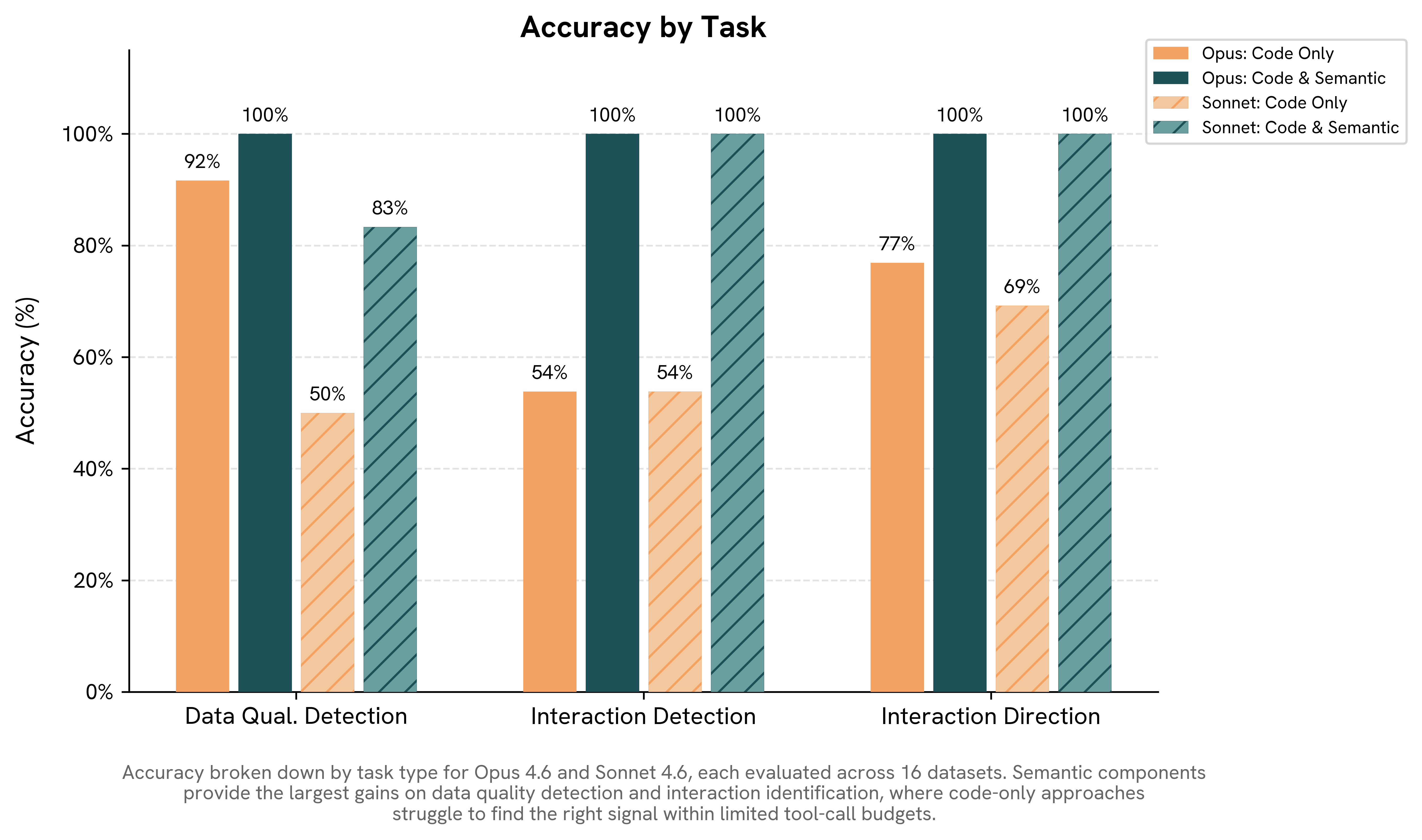
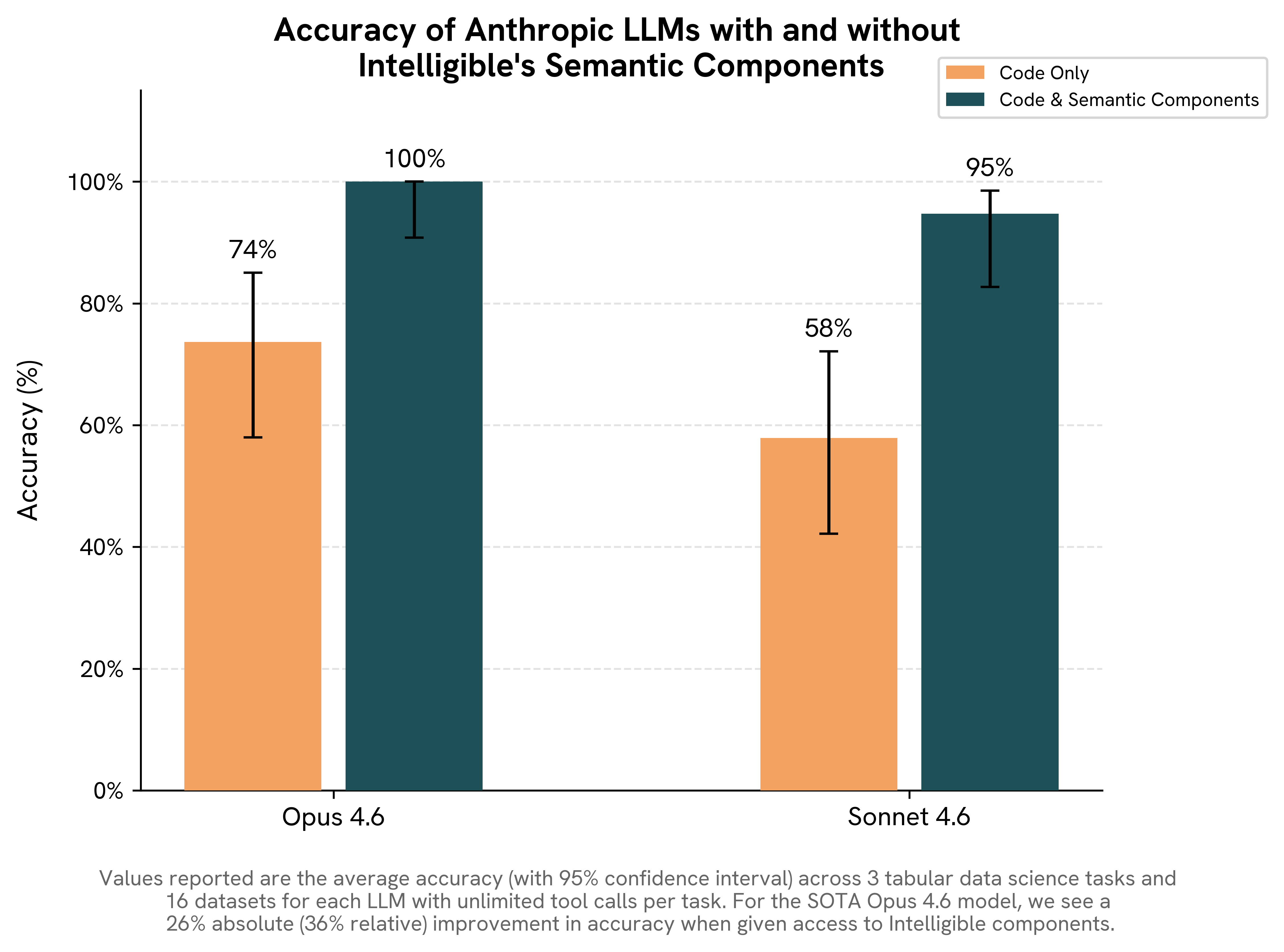
We evaluated this by presenting frontier LLMs with three analytical tasks under two conditions — with and without access to pre-computed structural knowledge — and measured how much that knowledge changed the accuracy of their answers.
‍

Setup

We gave the model a dataset, a Python sandbox, and an unlimited tool call budget, then asked it an analytical question. Each task runs in two conditions:

Code-only: The model can write and execute Python against the dataset. To assist the model, we pre-loaded the dataset into a Pandas dataframe in the Python sandbox.

Code + semantic components: The model also has access to pre-computed components (e.g. column summary statistics, feature importances, shape functions, pairwise interactions and interaction rankings from an Explainable Boosting Machine trained on the dataset). These components are automatically generated using Intelligible's intelligible-ai package and exposed to the model as callable tools — for example, get_feature_importances or get_interaction_rankings — that the model can invoke alongside its Python sandbox during the conversation.

The only variable across these two settings is whether pre-computed structural knowledge is available.

Within each of these two settings, we evaluated Claude Opus 4.6 and Claude Sonnet 4.6 across four base tabular datasets [1, 2, 3, 4] at multiple row counts (100, 500, 1,000, and 10,000). To avoid contamination from LLM training data, we constructed evaluation tasks by injecting a synthetic phenomenon (e.g., corrupted rows or artificial interactions) into a dataset. This ensured that the ground-truth answer (i.e., recovery of the injected phenomenon) was known, unambiguous, and unseen during training. In total, this procedure yielded 48 candidate tasks, of which 10 were excluded because the injected phenomenon was not sufficiently strong (e.g., an injected pairwise interaction did not rank as the strongest in the dataset), leaving 38 tasks for evaluation.

Task 1: Data Quality Detection

Task: A Boolean flag column marks problematic rows. Identify it. All column names are random strings.
‍

Why we care: In enterprise datasets, training on anomalous data silently degrades model performance. Identifying rules to exclude problematic rows is a routine but time-consuming part of data cleaning. Any AI system that is designed to deploy predictive models should first check for data quality.

Results:

Code-only accuracy (both models combined):

71%

With semantic components:

92%

Opus:

92%

100%

Sonnet:

50%

83%

For this task, we additionally obfuscate all column names with random strings. Frontier models have memorized popular tabular datasets. If you ask Claude about bike sharing data, it will recall column names and known quirks. Obfuscation ensures we’re measuring reasoning rather than recall.
‍

In code-only mode, the model explores ~20 opaque columns looking for the one that flags bad rows. It has no structural prior, so it falls back on heuristics: checking for missing values, high correlations, distribution anomalies.
‍

In contrast, when given Intelligible's semantic components, LLMs quickly identify the column that flags data quality problems. They do so by exploiting a nonobvious characteristic: data quality can be understood as an interaction effect, where a data quality indicator modulates the predictive relationship. In this task the indicator is a Boolean column in the dataset, so its two values produce clear differentials that surface as strong interaction effects.
‍

Armed with semantic components, the LLM follows a streamlined procedure. Opus, for example, typically needs just 4–6 calls: retrieve feature importances, examine the shape function of the top binary column, and confirm the result with a Python check.

Task 2: Interaction Detection

Task: Which pair of features has the strongest interaction effect on the outcome?
‍

Why we care: As the previous task showed, data quality problems can hide inside interaction effects. They're not the only thing hiding there—so do subgroup-specific risks, conditional treatment responses, and failure modes that only emerge when two conditions coincide. These patterns are invisible to linear methods, and they're exactly the patterns that drive costly surprises in production.

Results:

Code-only accuracy:

54%

With semantic components:

100%

Both Opus and Sonnet went:

54%

100%

Identifying interactions from scratch requires searching over all feature pairs, fitting interaction terms, computing H-statistics, or estimating SHAP values. These methods can find the right answer but also frequently disagree with the actual nonlinear interaction structure. Without a solid foundation to build on, LLMs identify the wrong pair on nearly half of instances, and different statistical methods produce different wrong answers.
‍

With semantic components, every single instance is solved in a single tool call. The LLM retrieves pairwise interaction rankings, reads the top-ranked pair, and answers. No Python needed.

Task 3: Interaction Direction

Task: For the strongest interacting feature pair: when the first feature (sorted alphabetically) is above its median, does increasing the second feature increase or decrease the outcome?
‍

Why we care: Knowing that two features interact is only half the picture. The direction determines whether the relationship is synergistic or antagonistic, and getting the direction wrong can invert a recommendation entirely.

Results:

Code-only accuracy:

73%

With semantic components:

100%

Opus:

77%

100%

Sonnet:

69%

100%

Comparing accuracies against Task 2 is misleading because this task is a binary question, so random guessing scores 50%.
‍

This task is a two-step problem: first identify the pair, then determine the direction. Code-only LLMs mostly fail on step one because they try to avoid the difficulty. Instead of exerting effort and employing complicated statistical tools to find the correct interaction pair, code-only LLMs use linear regression interaction terms, which leads to incorrect rankings and hence incorrect answers.
‍

With the semantic components, the harder subproblem (pair identification via retrieving interaction rankings) is precomputed and available as a tool call. Hence, the LLM focuses its Python code on what’s actually being asked: computing the conditional correlation. The typical pattern is 3 semantic calls (interaction rankings, dataset overview, interaction surface), followed by 2 Python calls (compute median, check direction). Five total calls, high accuracy.

The Full Picture

The pattern across these three tasks is consistent: when an analytical question depends on structural knowledge about the dataset, providing that knowledge as a pre-computed resource produces large accuracy gains.
‍

On one hand, this is obvious—giving a model more information should make it better at reasoning. On the other hand, it's surprising. None of the structural knowledge in these experiments was external to the datasets. Every answer was self-contained, derivable through statistical analysis of the data itself. We gave the LLMs an unlimited budget for Python calls. We weren't measuring efficiency; we were measuring accuracy. And yet, LLMs with Python sandboxes regularly got the wrong answer. Pre-computed semantic components produced major gains on questions the models could, in principle, have answered on their own.
‍

Reliable AI reasoning requires a foundation: persistent, precomputed knowledge about the data itself. This is what we're building at Intelligible. Our system extracts structural knowledge from enterprise data using interpretable models, persists it, and makes it available to LLMs and AI systems as an interactive semantic layer. The premise is straightforward: data meaning should be infrastructure, computed once and maintained, not regenerated from scratch on every query.
‍

These three tasks are a starting point. We're working on a full benchmark and associated tooling for evaluating grounded enterprise reasoning. If you're building in this space, let’s talk.

Aaron Alvarez is a research intern at Intelligible, supervised by Rich Caruana and Ben Lengerich. Questions or comments: rich@intelligible.ai.

Table of contents

Setup Task 1: Data Quality Detection Task 2: Interaction Detection Task 3: Interaction Direction The Full Picture

Stay in the loop.

Get product updates

Thank you! Your submission has been received!

Oops! Something went wrong while submitting the form.